Chapter 3. The simplest model with government money
Model SIM - Model SIMEX - A guide to Table 3.4
A more detailed guide to working out the numbers in table 3.4 on page 69 is available from the following file: Guide2Table3_4.pdf
Model SIMThere are two versions of model SIM used in the book, based on different starting values.
Version A of the program will generate model SIM, "starting with the beginning of the world",
to obtain results in Table 3.4, as described in par. 3.4.1, and figures 3.2 & 3.3,
discussed in par. 3.5.
Download: gl03sim_a (Eviews versions 5 to 8)
or gl03sim_a_v4 (Eviews 4.1)
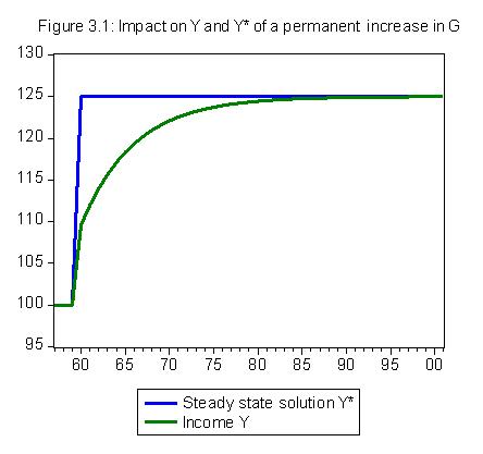
Version B of the program will generate model SIM, starting from steady state values,
to obtain results in figures 3.1 and 3.5, as discussed in par. 3.5 and 3.6.
Download: gl03sim_b (Eviews versions 5 to 8)
gl03sim_b_v4 (Eviews 4.1)
Version C of the program will generate model SIM, starting from steady state values,
to obtain results in figure 3.8, and study the effects of a change in the propensity to consume out of disposable income.
Download: gl03sim_c (Eviews versions 5 to 8) or
gl03sim_c_v4 (Eviews 4.1)
Version D of the program will generate model SIM, starting from steady state values,
to obtain results on the mean lag in the appendix.
Download: gl03sim_d (Eviews versions 5 to 8) or
gl03sim_d_v4 (Eviews 4.1)
Version A of the macro follows, with comments highlighted in green. |
 |
SIM_A for Eviews 5+
' Create a workfile, naming it SIM, to hold annual data from 1945 to 2010

wfcreate(wf=sim, page=annual) a 1945 2010

' Creates and documents series
series c_d
c_d.displayname Consumption goods demand by households
series c_s
c_s.displayname Consumption goods supply
series g_d
g_d.displayname Government goods, demand
series g_s
g_s.displayname Government goods, supply
series h_h
h_h.displayname Cash money held by households
series h_s
h_s.displayname Cash money supplied by government
series n_d
n_d.displayname Demand for labour
series n_s
n_s.displayname Supply of labour
series t_d
t_d.displayname Taxes, "demand"
series t_s
t_s.displayname Taxes, "supply"
series w
w.displayname Wage rate
series y
y.displayname Income = GDP
series yd
yd.displayname Disposable income of households

' Generate parameters
series alpha1
alpha1.displayname Propensity to consume out of income
series alpha2
alpha2.displayname Propensity to consume out of wealth
series theta
theta.displayname Tax rate

' Set sample size to all workfile range
smpl @all

' Assign values for
'   PARAMETERS
alpha1=0.6
alpha2=0.4
theta=0.2
'   EXOGENOUS
' note: government expenditure is zero up to 1954
smpl @first 1959
g_d=0
smpl 1960 @last
g_d=20
smpl @all
w=1
'   Starting values for stocks
h_h = 0
h_s = 0

' Create a model object, and name it sim_mod

model sim_mod

' Add equations to model SIM

' Equations which equalise demands and supplies
sim_mod.append c_s = c_d
sim_mod.append g_s = g_d
sim_mod.append t_s = t_d
sim_mod.append n_s = n_d

' Disposable income derived from accounting identity
sim_mod.append yd = w*n_s - t_s

' Tax payments
sim_mod.append t_d = theta*w*n_s

' Consumption function
sim_mod.append c_d = alpha1*yd + alpha2*h_h(-1)

' Increase in cash money, as a result of government deficit
sim_mod.append h_s = h_s(-1) + g_d - t_d

' Increase in cash held by households
sim_mod.append h_h = h_h(-1) + yd - c_d

' Determination of output
sim_mod.append y = c_s + g_s

' Determination of employment
sim_mod.append n_d = y/w

' End of model

' Select the baseline scenario

sim_mod.scenario baseline

' Solve the model for the current sample

sim_mod.solve


' Create variables for (simulated) changes in stocks
genr dh_s_0 = h_s_0 - h_s_0(-1)
genr dh_h_0 = h_h_0 - h_h_0(-1)

' Creates tables and charts from simulated variables

' Create Table 3.4 in the book from simulated values
table(13, 5) table3_4
table3_4(1,1) = "Table 3.4: The impact of $20 of government expenditure"
table3_4(3,1) = "Period"
setcell(table3_4, 3, 2, "1", "c")
setcell(table3_4, 3, 3, "2", "c")
setcell(table3_4, 3, 4, "3", "c")
setcell(table3_4, 3, 5, "n", "c")
setcell(table3_4,5,1,"G", "l")
setcell(table3_4, 6,1, "Y = G + C", "l")
setcell(table3_4, 7,1, "T = theta.Y", "l")
setcell(table3_4, 8,1, "YD = Y - T", "l")
setcell(table3_4, 9,1, "C = alpha1.YD+alpha2.H(-1)", "l")
setcell(table3_4, 10,1, "dHs = G - T", "l")
setcell(table3_4, 11,1, "dHh = YD - C", "l")
setcell(table3_4, 12,1, "H = dH + H(-1)", "l")
table3_4.setmerge(a1:e1)
table3_4.setwidth(1) 25
table3_4.setwidth(2:5) 6
table3_4.setlines(a4:e4) +d
!countvar = 0
for %var g_d y_0 t_d_0 yd_0 c_d_0 dh_s_0 dh_h_0 h_h_0
   !countvar=!countvar+1
   !count=0
   for %year 1959 1960 1961 2010
      !count = !count+1
      setcell(table3_4,4+!countvar,1+!count,@elem({%var}, %year), 0)
   next
next

show table3_4

' Creates the chart in Figure 3.2
smpl 1957 2001
graph fig3_2.line yd_0 c_d_0
fig3_2.setelem(1) lcolor(red) lwidth(2) lpat(2)
fig3_2.setelem(2) lcolor(green) lwidth(2) lpat(3)
fig3_2.name(1) Income YD
fig3_2.name(2) Consumption C
fig3_2.addtext(t) Figure 3.2: YD and C starting from scratch (table 3.4)
fig3_2.draw(line, left) 80

show fig3_2

' Creates the chart in Figure 3.3
smpl 1957 2001
graph fig3_3.line h_h_0 d(h_h_0)
fig3_3.setelem(1) lcolor(blue) lwidth(2) lpat(1)
fig3_3.setelem(2) lcolor(red) lwidth(2) lpat(3)
fig3_3.setelem(1) axis(right)
fig3_3.name(1) Wealth level H (money stock)
fig3_3.name(2) Household saving (the change in money stock)
fig3_3.addtext(t) Figure 3.3: Wealth level and wealth change, starting from scratch (table 3.4)
fig3_3.scale(left) linear range(0, 13) overlap
fig3_3.scale(right) linear range(0, 80) overlap

show fig3_3
Model SIMEX
Model SIMEX introduces expectations on households disposable income.
There are two versions of model SIMEX used in the book, based on different assumptions on expectations formation.
Version A of the program will generate model SIMEX, with expected disposable income equal to disposable income in the last period,
to obtain results in table 3.6 and figure 3.5 in the book.
Download: gl03simex_a (Eviews 5 to 8)
or gl03simex_a_v4 (Eviews 4.1)
Version B of the program will generate model SIM, assuming that expectations on disposable income are fixed,
to obtain results in figures 3.6 and 3.7.
Download: gl03simex_b (Eviews 5 to 8)
gl03simex_b_v4 (Eviews 4.1)