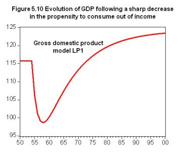
Model LP1
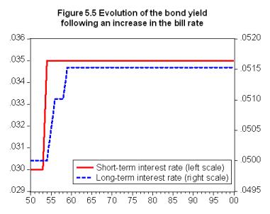
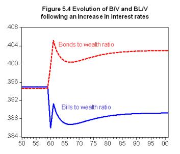
Model LP introduces government bonds as perpetuities, along with government bills. The chart shows the impact of a rise in the interest rates on both bills and bonds over households portfolio.
Download: gl05lp (Eviews 5 to 8) or gl05lp_v4 (Eviews 4.1)
model lp_mod

' Add equations to model LP

' Determination of output - eq. 5.1
lp_mod.append y = cons + g

' Regular disposable income - eq. 5.2
lp_mod.append yd_r = y - t + r_b(-1)*b_h(-1) + bl_h(-1)

' Tax payments - eq. 5.3
lp_mod.append t = theta*(y + r_b(-1)*b_h(-1) + bl_h(-1))

' Wealth accumulation - eq. 5.4
lp_mod.append v = v(-1) + (yd_r - cons) + cg

' Capital gains on bonds - eq. 5.5
lp_mod.append cg = (p_bl-p_bl(-1))*bl_h(-1)

' Consumption function - eq. 5.6
lp_mod.append cons = alpha1*yd_r_e + alpha2*v(-1)

' Expected wealth - eq. 5.7
lp_mod.append v_e = v(-1) + (yd_r_e - cons) + cg

' Cash money - eq. 5.8
lp_mod.append h_h = v - b_h - p_bl*bl_h

' Demand for cash - eq. 5.9
lp_mod.append h_d = v_e - b_d - p_bl*bl_d

' Demand for government bills - eq. 5.10
lp_mod.append b_d = v_e*(lambda20 + lambda22*r_b - lambda23*er_rbl - lambda24*(yd_r_e/v_e))

' Demand for government bonds - eq. 5.11
lp_mod.append bl_d = v_e*(lambda30 - lambda32*r_b + lambda33*er_rbl - lambda34*(yd_r_e/v_e))/p_bl

' Bills held by households - eq. 5.12
lp_mod.append b_h = b_d

' Bonds held by households - eq. 5.13
lp_mod.append bl_h = bl_d

' Supply of government bills - eq. 5.14
lp_mod.append b_s = b_s(-1) + (g + r_b(-1)*b_s(-1) + bl_s(-1)) - (t + r_b(-1)*b_cb(-1)) -p_bl*(bl_s-bl_s(-1))

' Supply of cash - eq. 5.15
lp_mod.append h_s = h_s(-1) + b_cb - b_cb(-1)

' Government bills held by the central bank - eq. 5.16
lp_mod.append b_cb = b_s - b_h

' Supply of government bonds - eq. 5.17
lp_mod.append bl_s = bl_h

' Expected rate of return on bonds - eq. 5.18
lp_mod.append er_rbl = r_bl+chi*(p_bl_e - p_bl)/p_bl

' Interest rate on bonds - eq. 5.19
lp_mod.append r_bl = 1/p_bl

' Expected price of bonds - eq. 5.20
lp_mod.append p_bl_e = p_bl

' Expected capital gains - eq. 5.21
lp_mod.append cg_e = chi*(p_bl_e - p_bl)*bl_h

' Expected regular disposable income - eq. 5.22
lp_mod.append yd_r_e = yd_r(-1)

' Interest rate on bills - eq. 5.23
lp_mod.append r_b = r_bar

' Price of bonds - eq. 5.24
lp_mod.append p_bl = p_bl_bar